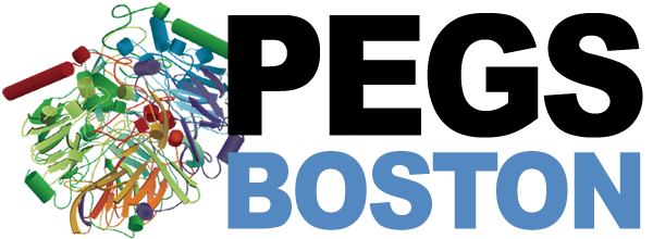
My favourite annual conference, PEGS Boston, ran from April 30 to May 4. For 14 years its logo and all related materials had featured the same protein, and for 13 years the organisers had been asking the same question: what protein is it? This year, the DVC team answered the question for the first time. The main question now is: how did we do it?
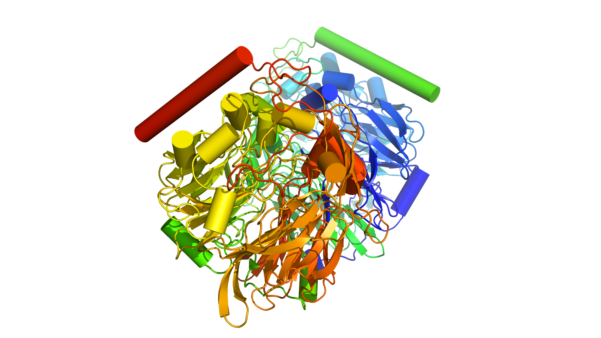
First, let us take a close look at the image. It is a cartoon representation of a protein in which the alpha helices are replaced with cylinders. In PyMOL, this appearance can be reproduced with the following settings:
show_as cartoon, all
set cartoon_fancy_helices, 0
set cartoon_cylindrical_helices, 1
The protein is also coloured using a spectrum distributed along the sequence. The very first amino acid is purple and the last is red. This takes one more simple command:
spectrum count, rainbow
We can now turn the standard all-atom representation
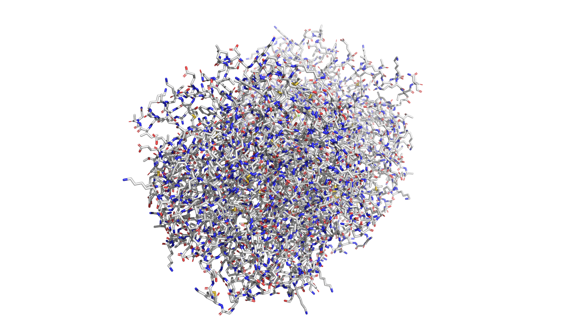
into a pleasant PEGS-style view
Our first idea was to generate images from the Protein Data Bank and compare them with our image using, for example, 2D Hamming distance. We later abandoned the idea—wrongly, as it turned out—but did end up with an image-generation script:
from pymol import cmd
import os

DIR = '/path/to/locate/pdbs'
IMG = '/path/to/store/images'

if not os.path.exists(IMG):
    os.mkdir(IMG)

for ent in os.listdir(DIR):
    filename = os.path.join(IMG, "%s.png" % ent)
    if os.path.exists(filename):
        continue
    cmd.load(os.path.join(DIR, ent))
    cmd.show_as('cartoon', 'all')
    cmd.set('cartoon_fancy_helices', 0)
    cmd.set('cartoon_cylindrical_helices', 1)
    cmd.spectrum('count', 'rainbow')
    cmd.orient()
    cmd.save(filename)
    cmd.reinitialize()
Running it in PyMOL's command-line mode is just as simple:
pymol -qc make_images.pyWe abandoned this idea because the current PDB simply contains too many entries. At the time of writing, the statistics were as follows:
| Experimental Method | Proteins | Nucleic Acids | Protein/NA Complex | Other | Total |
|---|---|---|---|---|---|
| X-Ray | 117481 | 1919 | 6011 | 10 | 125421 |
| NMR | 10708 | 1243 | 249 | 8 | 12208 |
| Electron Microscopy | 1546 | 31 | 542 | 0 | 2119 |
| Other | 215 | 4 | 6 | 13 | 238 |
| Multi Method | 116 | 4 | 2 | 1 | 123 |
| Total | 130066 | 3201 | 6810 | 32 | 140109 |
We did not know the correct orientation of the protein, and it could of course differ greatly from the one shown in the logo—the conference designers had surely rotated it. We therefore decided to begin filtering images by a few simple features that we could identify by eye.
It helped enormously that Sasha Nadolinsky recognised the image's creator and found a high-resolution version on his website. From that image, we concluded that we were looking for a single-chain protein containing at least 30 alpha helices, at least 17 of which were no more than five amino acids long. We also noticed an alpha helix at the beginning of the chain, so we decided to include that fact in our filters. The only uncertainty was whether the chain used the canonical blue-to-red colouring: besides the classic rainbow mode, there is also rainbow_rev, in which everything is reversed. There was a helix at the other end of the protein as well, though it did not begin right at the terminus. To be safe, we therefore specified that position 3 had to be covered by a helix.
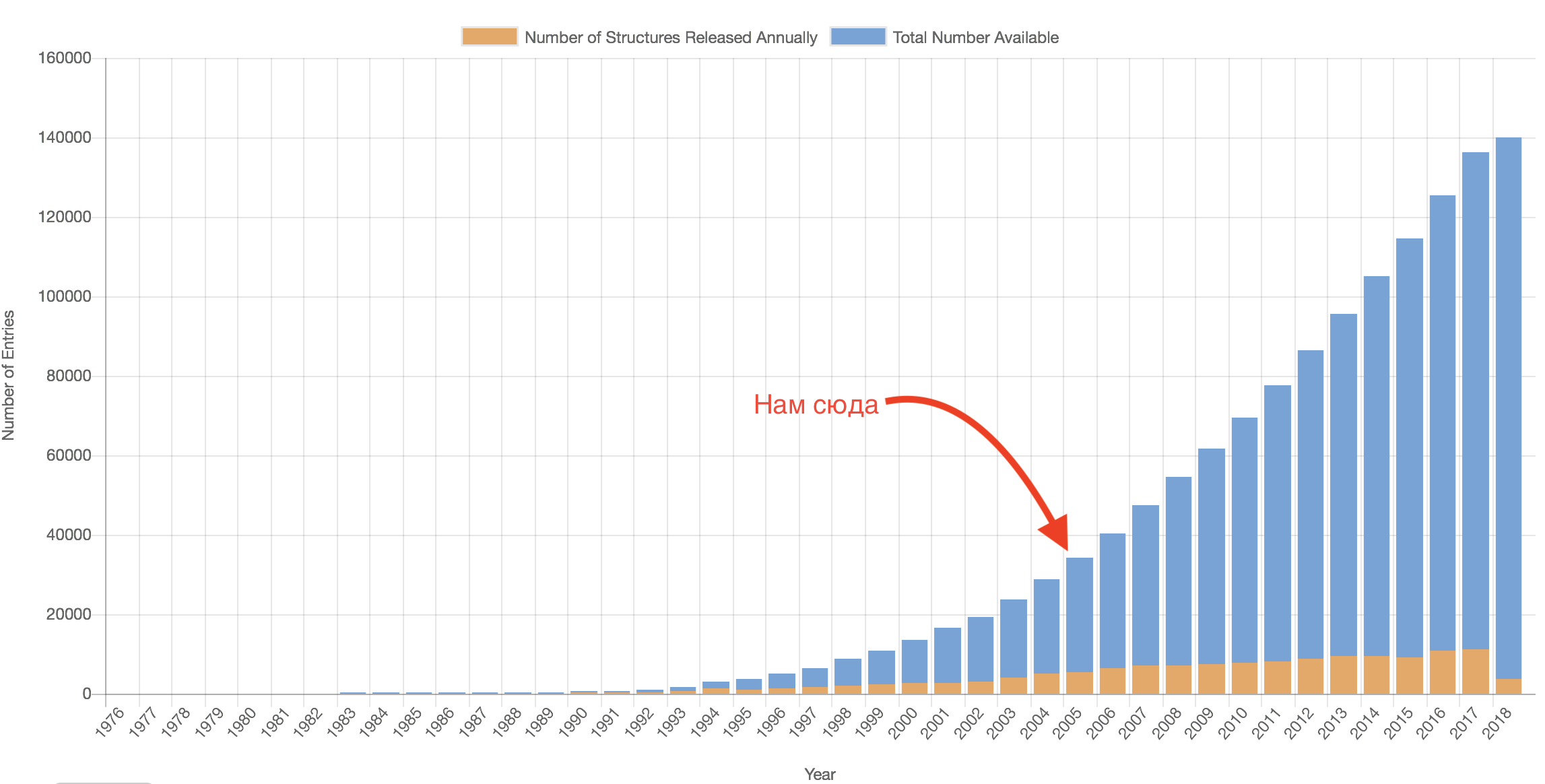
The main filtering criterion, of course, was the date: the first PEGS was held in 2005, so the protein must have been crystallised earlier. A look at the growth of the Protein Data Bank shows that this was by far the most powerful filter of all.
Let us begin. First, the entire Protein Data Bank has to be downloaded—we already had a local copy. Detailed instructions are available here, together with a convenient script for downloading everything using rsync. We need just one line from it, which downloads only the structures into their respective directories:
rsync -rlpt -v -z --delete --port=33444 rsync.wwpdb.org::ftp/data/structures/divided/pdb/ /path/to/your/local/dir > /tmp/pdb-download.log 2> /dev/nullThis gives us all 130,000-plus structures from the RCSB PDB. That sounds like a huge dataset, but we will process it using only primitive command-line tools to demonstrate otherwise. First, let us select all proteins deposited before 2005.
for filename in$(ls pdbs/*/*); do awk '$1 == "HEADER" {split($(NF-1),a,"-"); if (a[3] < 5 || a[3] > 18) {print FILENAME}}' $filename; done > pdbs_prior_2005.txtIn fact, the same code can be made considerably faster by using grep or ag for the initial filtering:
ag '^HEADER' pdbs | awk '{split($0,a,":"); split($(NF-1),b,"-"); if (b[3] < 5 || b[3] > 18) {print a[1]}}' > pdbs_prior_2005.txtOn a small set of 1,000 files, the difference looks like this:
time (for filename in$(ls pdbs/*/*); do awk '$1 == "HEADER" {split($(NF-1),a,"-"); if (a[3] < 5 || a[3] > 18) {print FILENAME}}' $filename; done > /dev/null)
3,45s user 1,84s system 98% cpu 56,206 total

time (grep -e '^HEADER' pdbs/* | awk '{split($0,a,":"); split($(NF-1),b,"-"); if (b[3] < 5 || b[3] > 18) {print a[1]}}' > /dev/null)
7,34s user 0,19s system 100% cpu 7,530 total

time (ag '^HEADER' pdbs | awk '{split($0,a,":"); split($(NF-1),b,"-"); if (b[3] < 5 || b[3] > 18) {print a[1]}}' > /dev/null)
0,70s user 0,30s system 278% cpu 0,358 total
Clearly, on a set of more than 130,000 files it pays to use ag 😉. Either way, we now have a file named pdbs_prior_2005.txt containing the paths of all files whose Protein Data Bank deposition date is earlier than 2005. As the chart above shows, the number of such structures is—
Now let us filter by the number of alpha helices. First, we will select all proteins containing 30 or more helices. This time, we will make the query efficient from the outset:
cat pdbs_prior_2005.txt | xargs ag "^HELIX 30" | awk '{split($0,a,":"); print a[1]}' > pdbs_p2005_h30.txtThe next task is to find 17 helices no more than five amino acids long. Once again, awk comes to our rescue, this time thanks to its ability to perform arithmetic:
for filename in$(cat pdbs_p2005_h30.txt);do ag "^HELIX" $filename | awk 'BEGIN{i=0}{ if ($9-$6 < 6) {i++} }END{ if (i > 16) { print "'$filename'" } }'; done > pdbs_ph_h17.txtWhat do we have at this point?
wc -l pdbs_ph_h17.txt
2537 pdbs_ph_h17.txt
The set is now a manageable size—only 2,537 entries—but that is still too many to examine by eye. Let us add the rule requiring the third amino acid to lie in an alpha helix:
cat pdbs_ph_h17.txt | xargs ag "^HELIX    1" | awk '($6 < 3) { split($1,a,":"); print a[1] }' > pdbs_phh_aa3.txt
wc -l pdbs_phh_aa3.txt
142 pdbs_phh_aa3.txt
Now we have just 142 structures!
After inspecting every one of them, we identified the structure we needed: 1G72, number 117 in the list. As it turned out, the image on the RCSB website has exactly the same orientation as the conference logo, so our original Hamming-distance idea would have worked perfectly. But this was an excellent opportunity to practise using command-line tools on “big” data.